IMPACT OF SAFTA ON SOUTH ASIAN TRADE

Ram K. Regmi¹ --- Satis C. Devkota² --- Mukti P. Upadhyay³⁺

¹Statistical Officer, Ministry of Finance, Kathmandu, Nepal
² Assistant Professor of Economics and Management, University of Minnesota - Morris
³Professor of Economics, Eastern Illinois University

Keywords:Regional trading bloc, SAFTA, Trade creation, Trade diversion, Gravity model.

JEL Classification: F14, F15, O53.

ARTICLE HISTORY: Received:18 October 2016 Revised:21 November 2016 Accepted:25 November 2016Published:29 November 2016

1. INTRODUCTION

Realizing the need for greater economic integration for faster economic growth, South Asian countries—Nepal, India, Bangladesh, Bhutan, Pakistan, Sri Lanka, and Maldives—signed an agreement in 1985 to establish the South Asian Association for Regional Cooperation (SAARC). The region started to move away from their inward-looking import substitution policy when Sri Lanka initiated to liberalize its economy during early 1980s followed by India in the early 1990s and others about the same time. The formation of SAARC led to partial removal of the existing trade barriers among members resulting in the launch of the South Asian Preferential Trade Arrangement (SAPTA) in December 1995. Further commitment to regional integration occurred in 2006 with the establishment of South Asian Free Trade Area (SAFTA). While a deeper integration effort has not materialized since then, intra-regional trade in South Asia continues to show progress.

A gravity model can be an effective tool in understanding the depth of trading relationships among countries. According to Arkolakis et al. (2012) “estimating the trade elasticity using a gravity equation is a particularly attractive procedure since, by its very nature, it captures by how much aggregate trade flows, and therefore consumption, reacts to changes in trade costs.”

Table 1.1 shows the distribution of nominal intra-regional exports in South Asia from 1981 to 2010 in five-year averages. Shares for India and Pakistan, the largest economies, set the average regional pattern that reflects modest intraregional exports. Bangladesh experienced the largest decline of export share, driven by its greater export concentration outside the region in developed countries.

Table-1.1. Regional Exports as a Share of Total Exports of South Asia (in percent)

Country	1981-85	1986-90	1991-95	1996-00	2001-05	2006-10
Bangladesh	8.81	4.54	2.87	2.07	1.71	2.55
India	3	4.08	2.97	4.61	5.35	4.88
Maldives	18.85	14.63	24.65	17.93	16.34	16.62
Nepal	52.36	18.2	7.91	30.95	57.56	68.64
Pakistan	4.53	3.94	3.6	3.37	3.27	3.86
Sri Lanka	6.4	4.94	2.59	2.84	6.93	7.47
South Asia	4.36	3.58	3.86	4.32	5.3	4.98

Source:- IMF-DOTS, 2015.

The highest intra-regional export share went to Nepal, primarily due to India’s dominance in Nepal’s trade. This share even grew in the last two five-year periods reaching a peak of 69 percent. Maldives, the smallest country in the region, and Sri Lanka also posted higher shares than the regional average. It is noteworthy that India’s economic size and dominance in the region has grown further in recent decades. India already accounted for 60 percent of total exports within the region during the 1980s but its share jumped further to about 80 percent during 2000s.

Table-1.2. Regional Imports as a Share of Total Imports in South Asia (in percent)

Country	1981-85	1986-90	1991-95	1996-00	2001-05	2006-10
Bangladesh	3.36	4.94	12.06	14.27	15.52	15.21
India	0.83	0.44	0.57	0.77	0.92	0.67
Maldives	14.49	10.81	15.03	21.45	22.57	13.63
Nepal	34.68	18.41	17.76	28.86	51.53	60.2
Pakistan	1.9	1.73	1.51	2.22	2.65	4.79
Sri Lanka	6.24	7.13	11.26	11.27	17.52	22.76
South Asia	2.08	1.93	3.23	4.08	4.32	3.45

Source:- IMF-DOTS, 2015.

Table 1.2 highlights imports within South Asia. Compared with exports the import concentration has been fairly low throughout the study period. However, imports show a growing pattern after 1995 following the SAPTA implementation. Once again, Nepal had the highest share of its imports from regional partners and it was because of its closest and even increasing trade relationship with India, particularly after 2000. Bangladesh also shows a rise from about 3 percent in the beginning to about 15 percent at the end of the sample period. Maldives remained between 10 and 20 percent, Pakistan showed a rising trend, and Sri Lanka not only increased its intra-regional imports but stayed above the regional average. In contrast, India’s import share has stood fairly low, below 1 percent as well as below the regional average, throughout the last 30 years. Yet, India’s size again makes the country the largest importer from within the region, equal to 60 percent in the 1980s and rising to nearly 80 percent in the year 2010.  Figure 1 shows the direction of exports within the SAARC region and without. Figure 2 then shows the trend on the import side. Both figures show growth of intra-regional trade being higher than growth of inter-regional trade and indicate the possibility of a greater role of liberal trade policies within the region during the SAPTA and SAFTA periods. Next, Tables 2.1 and 2.2 indicate the distribution of South Asia’s trade in five-year intervals with five other geographical regions: the rest of Asia (and Oceania), Europe, North America, Latin America, and Africa.  Figures 1 and 2 show that Asia, Europe, and North America are South Asia’s major trading partners. Rest of Asia stands as a largest trading regional bloc while Latin America remains the smallest.

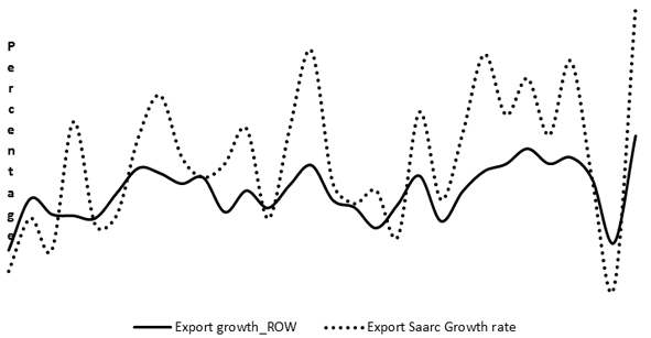
Figure-1. Annual Change in Exports: Rest of the World and SAARC

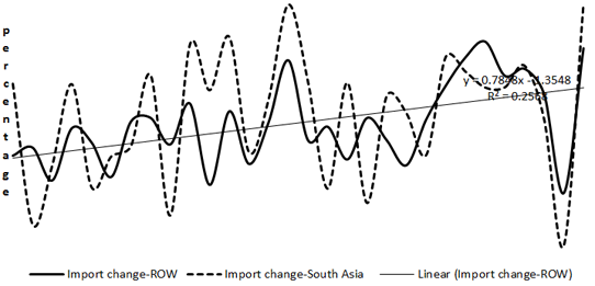
Figure-2. Annual Change in Imports: South Asia and Rest of the World

Recent data suggest that South Asia’s increasing trade concentration in the rest of Asia has displaced trade with North America. While North America, led by the United States, takes in about 20 percent of South Asia’s exports, South Asian imports from North America have plummeted from 15 percent in 1985 to 6 percent in 2010. At the same time, South Asia’s imports from the rest of Asia grew from 48 to 62 percent between 1985 and 2010. Europe-plus, which includes nations in the former Soviet Union, is the second largest export market for South Asia, covering between 26 and 39 percent of total share. Likewise, this trading bloc supplies 20 to 30 percent of South Asia’s imports. Latin America, on the other hand, registered as least integrated trading bloc for South Asia with a trade share of 1 to3 percent. Africa has performed slightly better than Latin America with its export and import shares between 3 and 10 percent.

Trade statistics described above indicates that South Asia has been a moderate rather than heavy trader with rest of the world. This raises the question of how much trade has increased as a result of SAFTA within the South Asian region and with other regions of the world.

2. BRIEF REVIEW OF LITERATURE

For half a century, the gravity equation has been used to estimate the ex post partial effects of regional trade agreements, among other factors, on bilateral trade flows (cf., (Tang, 2005; Anderson, 2011; Bergstrand and Egger, 2011) for recent surveys). Eichengreen and Irwin (1998) termed the gravity model as a “workhorse,” indicating its success in terms of high explanatory power, and relatively stable estimated coefficients, based on the application of data sources that were readily available. Theoretical foundation of the model can be traced back to Anderson (1979) and Bergstrand (1985;1989) who first developed micro-foundations for the gravity equation. Subsequent refinements were added by several economists. Helpman and Krugman (1985) argue that gravity models reflect more of trade in differentiated products by countries at similar income levels. Deardorff (1995) asserts that a gravity model can be derived from any one of multiple hypotheses about trade, and hence is suitable to testing any one of them.
We refer to more studies in the literature while discussing the formulation and estimation of our model in the next section.

3. ESTIMATION METHOD AND DATA

3.1. Estimation Method

In the gravity equation, the key trade creation variable is a dummy equal to one if two trading countries are members of a common RTA (Regional Trade Agreement) and zero otherwise. A positive coefficient for the dummy indicates creation of additional trade caused by forging of the RTA after carefully controlling for other factors that possibly affect bilateral trade.  A negative sign for the dummy is the indication that the RTA decreases trade. With regard to capturing the extra-regional trade behavior, we interact each period dummy to the RTA dummy of other five regional trading blocs. Since South Asian RTA was created in 1995, our period dummy equals one if the observations are for 1995 through 2010 and equals zero for years before 1995. The coefficients of these interaction dummies are thus expected to reveal extra-regional impact of SAPTA/SAFTA. Including other standard gravity controls we obtain our estimating model as follows:

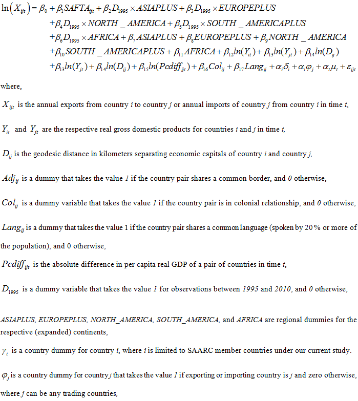
Having a common language in two countries is historically associated with closer ties between the firms of trading countries helping trade expansion. Colonial relationships through, for example, membership in British Commonwealth may provide cultural familiarity among nations enhancing commercial ties. Similarly, countries sharing a common border will likely have a lower trade costs relative to those without common borders. Thus, the coefficients of language and colonial relationship are expected to be positive, while distance should have a negative coefficient. Finally, difference in per capita incomes is included to test Linder’s hypothesis that countries with high and similar incomes trade more. The sign of its coefficient, β15, cannot, however, be established a priori. Similarity of incomes among richer countries may bring the structure of product demands closer together causing greater trade in similar products. But large income differences between rich and poor countries can also increase trade but in dissimilar products.

3.2. Estimation Issues

The gravity model was significantly enhanced by Anderson and Van-Wincoop (2003) who introduced the concept of “multilateral trade resistance” (MTR). Natural and other trade barriers between two countries, say Nepal and India, can be summarized under bilateral trade resistance. But if a third country, say Japan, liberalized its trade with India, then it would reduce MTR of India (may be slightly because India also trades with many other countries) which in turn would divert some of Nepal-India trade to trade between India and Japan. Thus trade between Nepal and India not only depends on their bilateral trading cost but rather on this cost relative to the cost of each country when it trades with the rest of the world, i.e., their MTRs.

Thus, in our example, Japan’s liberalization with India has implications for Nepal-India trade and this factor must be included in the model to avoid the upward bias that would otherwise result in the effects of RTA and other factors. As Feenstra (2004); Baier and Bergstrand (2007) and Florin et al. (2007) show, however, MTR’s effect can be controlled by using country fixed effects in a cross-section framework. The fixed effects parameters will also capture other country-specific time-invariant determinants of trade not picked up by other controls. This is also helpful to our model because the tariff data were not available for many countries for many years and even the available data were mostly the average rates justifying exclusion of the variable altogether.

Furthermore, by extending the cross section for 31 years of data that we use in our panel model, we also address the possible fragility of the estimates  discussed by Ghosh and Yamrik (2004). Finally, in a time series of over 30 years, a failure to control for global economic shocks such as large swings in the oil price or global inflation can cause omitted variable bias in the estimates (Baldwin and Taglioni, 2006). We therefore add time dummies to capture potential global economic shocks in the model.

Finally, some endogeneity of GDP as an expanatory variable may not be avoidable because GDP partly depends on net exports, the dependent variable. However, the use of labor, physical capital and human capital as instruments for GDP has meant little difference in results (Frankel et al., 1998). The most common problem of IV techniques in gravity equation using cross-section data is failure to find acceptable intruments.

3.3. Data

This study uses secondary data. Bilateral exports and imports flows of merchandise goods are taken from the International Monetary Fund’s Direction of Trade Statistics (DOTS). Nominal exports and imports are in their f.o.b.¹ and c.i.f.² values respectively in US dollars and are converted into real dollars by using the US GDP deflators. GDP and GDP per capita are in 2005 PPP international US dollars and taken from the World Development Indicators online (World Bank).

The trading partner countries are chosen from the ISO-alpha-3³ classification consisting of 225 countries. Exports and imports for the seven SAARC countries (Bangladesh, Bhutan, India, Maldives, Nepal, Pakistan, and Sri Lanka) are taken as our potential primary sample. Unfortunately, data for Bhutan is limited only in the form of partners’ data rather than data from Bhutan as a reporting country.  Thus, we are left with 41,664 (6 × 224 × 31) observations as the maximum number of possible observations of bilateral exports/imports covering years 1980-2010. Most of the variables of interest are also missing for 52 iso3-coded countries. Dropping these countries leaves 166 partner countries of SAFTA in the sample. Missing values on several variables for some countries again reduced observations to 22,310 for exports and 21,806 for imports. Tables 3.1 and 3.2 present the summary statistics used for estimating real exports and real imports.

Data on geographical distance, contiguity, colonial relationships, and language are extracted from Centre d’Etudes Prospectives et d’Informations Internationales (CEPII)⁴ database. Distance data refer to the distance between the two most populated cities, one for each country. CEPII uses the great circle formula to calculate the geographic distance between countries, referenced by latitudes and longitudes of the largest agglomerations in terms of population.

Obviously many bilateral trade data suffer from zero values. This could be due to true zero trade, small trade numbers reported as zeros or missing data mistakenly reported as zeros.  Literature shows several alternative ways to handle the zero problem in the log-linear specifications of the model. But as Baldwin and Harrigan (2007) and Wang and Winter (1991) have shown, the choice of methods has no substantial effect on estimation results. In this study, we add the constant 1 to each dependent variable.

4. RESULTS AND DISCUSSION

This section discusses results for real exports and real imports separately as the behavior of bilateral trade can differ substantially among the two components.

4.1. Export Performance

Table 4 shows the results for exports under different specifications of the model. Effect of the SAFTA formation appears on row 1. Column (1) gives the results of the baseline model, as in Frankel (1997) where non-SAFTA trade areas are not controlled for. The SAFTA coefficient suggests a country pair exports about ((e0.162-1)×100=) 18 percent more than a pair of otherwise similar non-member countries, after controlling for other factors. Other dummies have the expected signs and are statistically different from zero. Cultural and to some extent political ties represented by shared language and previous colonial relationships are important export promoting  factors. Additional exports between the member countries is also attributable if they share a common border. As hypothesized, a difference between per capita incomes does not seem to matter since its coefficient is statistically insignificant although the high R2 supports  the fit of the model reasonably well.

Table-4. Gravity Results for Exports with Panel Data: 1980-2010

Dependent variable: Log Exportijt
	Linear					Tobit
	-1	-2	-3	-4	-5	-6
SAFTAij	0.162***	0.204***	0.22***	0.205***	0.241**	0.169***
	-0.032	-0.028	-0.035	-0.041	-0.098	-0.045
ASIAPLUS×D1995	-	0.061***	0.084***	0.06***	0.133***	0.045
		-0.013	-0.029	-0.027	-0.049	-0.032
EUROPEPLUS×D1995	-	0.085***	0.108***	0.146***	0.199***	0.14***
		-0.012	-0.031	-0.028	-0.045	-0.032
NORTH  AMERICA×D1995	-	0.29***	0.31***	0.277***	0.425***	0.335***
		-0.07	-0.066	-0.046	-0.108	-0.047
SOUTH AMERICAPLUS×D1995	-	-0.013	0.011	-0.019	-0.043	-0.045
		-0.009	-0.028	-0.026	-0.032	-0.032
AFRICA×D1995	-	-0.018**	0.005	-0.013	-0.029	-0.073**
		-0.007	-0.028	-0.026	-0.034	-0.031
ASIAPLUS	-	0.019	0.011	-0.938***	-	0.26***
		-0.014	-0.016	-0.213		-0.044
EUROPEPLUS	-	-0.11***	-0.117***	-1.634***	-	-0.366***
		-0.016	-0.018	-0.169		-0.062
NORTH  AMERICA	-	0.137***	0.131***	0.15*	-	1.287***
		-0.042	-0.04	-0.06		-0.14
SOUTH AMERICAPLUS	-	-0.097***	-0.108***	-0.922***	-	-0.189***
		-0.015	-0.018	-0.209		-0.06
AFRICA	-	0.017	-0.06	-1.31***	-	0.322***
		-0.013	-0.016	-0.152		-0.041
Log GDPit	1.335***	0.125***	0.124***	1.3454**	1.43***	1.67***
	-0.059	-0.002	-0.002	-0.059	-0.134	-0.064
Log GDPjt	0.113***	0.109***	0.109***	0.132***	0.127***	0.198***
	-0.015	-0.002	-0.002	-0.015	-0.039	-0.019
Log Distanceij	-0.062***	-0.02	-0.019***	-0.068***	-	0.087***
	-0.015	-0.007	-0.007	-0.015		-0.018
Log Per Capita Differenceijt	0.001	0.0327***	0.036***	0.001	0.002	-0.009**
	-0.002	-0.002	-0.002	-0.002	-0.01	-0.003
Languageij	0.023*	0.13***	0.131***	0.0221*	-	0.063***
	-0.012	-0.011	-0.011	-0.012		-0.014
ADJij	0.487***	0.328***	0.327***	0.483***	-	0.336***
	-0.046	-0.049	-0.049	-0.045		-0.044
Colonyij	1.282***	1.087***	1.08***	1.28**	-	0.993***
	-0.067	-0.062	-0.062	-0.068		-0.058
Constant	-35.458***	-5.76	-5.67***	-34.55***	-38.21**	-45.39***
	-1.595	-0.124	-0.124	-1.6	-3.726	-1.7
Year  Dummies	Yes	No	yes	Yes	Yes	Yes
Country Dummies	Yes	No	No	Yes	No	Yes
Country-Pair Dummies	No	No	No	No	Yes	No
Total Observations	22,310	22,310	22,310	22,310	22,310	22,310
R2	0.6128	0.444	0.446	0.6164	-
No. of Uncensored Observations	-	-	-	-	-	15,945
No. of Censored Observations	-	-	-	-	-	6,365
Log Pseudo-likelihood	-	-	-	-	-	-8,938

Source:- Calculated by Authors, 2015.
Note: Robust standard errors are in parentheses. Statistical significance at 1%, 5% or 10% level are indicated by ***,** or *, respectively. Coefficients estimates for exporter/importer and time effects are not reported for brevity.

When other controls are included, the results, as shown in columns 2, 3 and 4 of Table 4, retain the significance of our key variable of interest, SAFTA. That is, whether we account for any time-varying characteristics across countries or time-invariant characterists within countries, the impact of the SAFTA membership on trade is almost unaltered, in terms of the sign, statistical significance and even mostly the magnitude of the effects.

Thus, for example, the SAFTA coefficient on column 4 suggests that two SAFTA countries on average export 23 percent (e0.205-1)×100) more than two otherwise similar non-member countries. The SAFTA coefficients in columns 2, 3 and 4 range between 0.205 and 0.241.

Looking at the coefficients of other regional blocs, three regions—ASIAPLUS, EUROPEPLUS and NORTH_AMERICA—are observed to be export creating blocs for South Asia. The ASIAPLUS comprises China, Japan, Australia, the Middle East, and members of the ASEAN. The interaction of these regions with D95, the South Asian dummy for the year in which SAFTA was created and after, shows that South Asia’s exports to ASIAPLUS increased further after the formation of SAFTA though the magnitude shows the effect is marginal. The European region and North America exhibit strong export growth for South Asia. Indeed, with North America, a 32 percent (=(exp(0.277)-1)×100) average growth is higher than intra-SAFTA export growth and could be attributed to the US’s unilateral trade liberalization and the special privilege extended to South Asian export quotas on garments.

On the contrary, Latin America and Africa do not show a positive impact. Because of low and unstable share of the South Asia’s trade with these regions, the corresponding coefficients are both negative and statistically insignificant.

Among control variables, GDPs of exporting and importing countries are  important export determinants, as is the case with most of the gravity results in the literature. Second, our gravity variable is geographical distance which proxies for natural trade cost and shows its usual negative sign. A country that is, say, 20 percent closer to another than it is to a third country is likely to have 1.4 percent more exports with that second country. Third, having a common language, sharing common borders, and having formal colonial relationships appear to be export promoting factors. While each of these factors are significant, colonial impact dominates others. Column (4) in Table 4 shows that exports between a country pair increased 2.5 percent (=(exp(1.28)-1)×100) if the two countries had a colonial relationship compared to another otherwise similar country pair with no such relationship. Note that most of the SAARC countries were formerly United Kingdom colonies. On the other hand, the variable per capita income difference is no longer a factor behind exports, after we have controlled for country-specific characteristics and global economic fluctuations. Overall, the evidence at our disposal is unable to distinguish whether the exports follow the predictions of the Heckher-Ohlin model or the new trade theory. Most of the country dummies as well as regional dummies are statistically different from zero indicating the country and region specific characteristics provide an important influence on exports.

Our results on exports are closer to Delgado (2007) who finds a minor but significant effect of SAFTA on regional trade, and Srinivasan (1994) who finds a larger regional effect from trade liberalization.

4.2. Import Performance

Potential trade diversion away from the non-member countries can be tested by estimating simultaneously the effects on both intra- and extra-SAFTA imports. We therefore rerun equation (1) for imports, and the estimated results are presented in Table 5.

Table-5. Gravity Results for Imports with Panel Data:1980-2010

Dependent variable: Log Importijt
	Linear					Tobit
	-1	-2	-3	-4	-5	-6
SAFTAij	0.181***	0.156***	0.138***	0.222***	0.251**	0.127**
	-0.033	-0.028	-0.033	-0.042	-0.124	-0.056
ASIAPLUS×D1995	-	0.078***	0.056	0.13***	0.275***	0.094**
		-0.017	-0.028	-0.028	-0.054	-0.043
EUROPEPLUS×D1995	-	-0.002	-0.026	0.058***	0.07*	0.003
		-0.013	-0.028	-0.028	-0.041	-0.043
NORTH  AMERICA×D1995	-	-0.061	-0.078	-0.019	0.068	-0.051
		-0.059	-0.055	-0.045	-0.047	-0.054
SOUTH AMERICAPLUS×D1995	-	-0.047***	-0.068**	-0.024	-0.065*	-0.048
		-0.01	-0.02	-0.027	-0.036	-0.044
AFRICA×D1995	-	-0.056**	-0.077***	-0.022	-0.043	-0.068*
		-0.009	-0.025	-0.026	-0.038	-0.041
Log GDPit	1.042***	0.127***	0.126***	1.051***	1.12***	1.5***
	-0.069	-0.002	-0.002	-0.069	-0.137	-0.076
Log GDPjt	0.242***	0.144***	0.143***	0.214***	0.206***	0.328***
	-0.019	-0.002	-0.002	-0.019	-0.047	(0.026
Log Distanceij	-0.23***	-0.066***	-0.068***	-0.234***		0.318***
	-0.016	-0.008	-0.008	-0.016		-0.02
Log per capita Differenceijt	0.008***	0.056***	0.058***	0.01***	0.0004	0.009*
	-0.003	-0.002	-0.002	-0.003	-0.011	-0.005
Languageij	-0.039***	0.09***	0.09***	-0.038***	-	0.005
	-0.014	-0.013	-0.013	-0.014		-0.019
ADJij	-0.037	0.348***	0.348***	-0.036	-	-0.273***
	-0.046	-0.051	-0.051	-0.046		-0.043
Colonyij	1.095***	0.916***	0.916***	1.094***	-	0.773***
	-0.069	-0.063	-0.063	-0.069		-0.058
ASIAPLUS	-	0.188***	0.198***	0.433***	-	-0.236***
		-0.016	-0.018	-0.062		-0.041
EUROPEPLUS	-	-0.129***	-0.118***	-0.402***	-	0.533***
		-0.016	-0.019	-0.085		-0.12
NORTH AMERICA	-	0.09**	0.099**	0.475**	-	0.2
		-0.04	-0.039	-0.205		-0.182
SOUTH AMERICAPLUS	-	-0.021	-0.012	0.74***	-	-0.481***
		-0.015	-0.019	-0.066		-0.095
AFRICA	-	0.078***	0.085***	-0.258	-	0.4***
		-0.013	-0.017	-0.175		-0.052
Constant	-29.35***	-6.42***	-6.29***	-28.94	-32.5	-42.37***
	-1.822	-0.142	-0.141	-1.77	-3.73	-2.02
Year Dummies	Yes	No	Yes	Yes	Yes	yes
Country Dummies	Yes	No	No	Yes	No	yes
Country-Pair Dummies	No	No	No	No	Yes	No
Total Observations	21,806	21,806	21,806	21,806	21,806	21,806
R2	0.6068	0.4471	0.4508	0.6219	-	-
No. of Uncensored Observations	-	-	-	-	-	14,090
No. of Censored Observations	-	-	-	-	-	7,716
Log Pseudo-likelihood	-	-	-	-	-	-11168.11

Source:- Calculated by Authors, 2015.
Note: Robust standard errors are shown in parentheses. Statistical significance at 1%, 5% or 10% level are indicated by ***,** or *, respectively. Coefficient estimates for exporter/importer and time-specific effects are not reported for brevity.

As with exports, the SAFTA coefficient has a significant and positive effect on the imports originating in the member countries (column 1). Imports among the SAARC member countries grew about 20 percent (= exp(0.181)-1)×100) compared to otherwise similar but non-member country pairs. Other control variables generally have coefficients that show expected signs and significance. For instance, importing and exporting countries’ income elasticities of imports are positive, in line with the theory. Distance, as usual, works as a trade reducing factor. Colonial relationships have a strong effect on import volumes, as we found for exports in Table 4. Surprisingly, however, sharing a language now turns out to be an import hindering factor, contradicting our expectation.

The SAFTA coefficients across column (2) through column (4) are all positive and significant. Dropping the year-specific (column 2) and country-specific unobserved fixed effects, SAFTA is expanding intra-regional imports by about 17 percent (=exp(0.156)-1) ×100). The effect declines slightly to about 15 percent once the time trend is controlled for (column 3).

Column 4 of Table 5 presents results after controlling for heterogeneity across years and countries. SAFTA’s coefficient of 0.222 suggests an additional imports of about 25 percent between member country pairs than are imports from outsiders, holding other factors constant. The non-SAFTA effect is captured by the coefficients of other regional dummies interacted with the period dummy, D1995. The coefficients of ASIAPLUS and EUROPEPLUS are positive and statistically significant. This suggests that after forming the South Asian trade bloc, imports originating from these countries have indeed grown. However, imports from North America, Latin America, and Africa seem irrelevant at any conventional significance level. In summary, the evidence suggests that SAFTA has not hindered imports from other countries, or provided favors to the inefficient suppliers within the region.

Basic gravity controls such as GDPs of importing and exporting countries are positively import elastic (column 4, Table 5). Bilateral distance, as usual, proves to be an import hindering factor: greater the distance, smaller the imports. A country seems to be importing 2.3 percent less if it is 10 percent farther from the exporting country. A shared colonial history means larger imports, as well as larger exports as we saw in the last subsection. Imports were twice as large for two countries linked by colonial relationship as for those unrelated in this way. Sharing a common language has the unexpected negative effect. On the other hand, having a common border seems less problematic for its negative sign since its coefficient is statistically insignificant.

Absolute difference in per capita incomes remains positively related with real imports (column 4). The Heckscher-Ohlin model predicts greater trade betweeen countries with different factor endowments since endowment differences are generally related with differences in per capita incomes.⁵ South Asian countries lag far behind developed countries in the stock of capital per unit of labor. As a result, they rely on the import of capital or capital-intensive goods from developed countries such as Japan, Korea, Europe and the USA.
To conclude, our panel regressions overwhelmingly support our hypothesis that SAFTA is import creating. These results are generally consistent with many gravity results in the literature, such as the findings in Hiranatha (2004); Coulibaly (2004); Rahman et al. (2006); ADB and UNCTAD (2008) and Delgado (2007). Furthermore, a recent study undertaken by Acharya et al. (2010) shows that along with many RTAs, SAFTA is an intra-trade, extra-export, and extra-import creating trade bloc.

4.3. Robustness Test

To measure the robustness of our estimated equations, we estimate the exports and imports separately using different methods. First, the regressions still use fixed effects but the fixed effects are now applied to country pairs rather than to individual countries. The results of this exercise appear in column (5) of both Tables 4 and 5. The directions of the coefficients are unchanged for exports (Table 4) with little variation in magnitudes. Intra-bloc and extra-bloc export effects are consistent with our earlier results in Table 4 (column 4). Similarly, the SAFTA coefficients on the import equation also remain the same. Other regional effects are also similar except for South America for which the results indicate the existence of trade diversion.

Some of the gravity studies in the literature favor Tobit estimation in the presence of many zeros that are presumably distributed non-randomly. We test our results using this method as well. The estimated coefficients appear in column 6 of Table 4 and Table 5. The SAFTA coefficients in all the cases are again positively significant and are consistent with our earlier results. Asia, the European area, North America, and South America indicate no change for both exports and imports. The African territory is now the exception with significantly negative effects for exports as well as imports. We conclude that our results remain fairly robust to alternative econometric considerations.

5. CONCLUSION

In the context of contradictory results that we observe in the literature for the South Asian trade bloc, this empirical study provides a careful examination of data to demonstrate the effects of SAFTA on trade. Using a wide range of country panels covering the recent 31 annual observations, our gravity model finds SAFTA to be indeed a trade creating regional bloc in both exports and imports. We test simultaneously the intra-trade and extra-trade effects. Intra-bloc exports are stimulated on average by 23 percent because of SAFTA, while intra-bloc imports rise by 25 percent. 

The test of whether SAFTA has created or diverted trade on the net clearly shows that SAFTA is indeed a net trade-creating bloc. The Asian, European, and North American regions responded affirmatively to the SAFTA bloc.  For exports, the increase in the North American market is higher than the increase within South Asia itself whereas the South American region and African continent are virtually non-responsive to SAFTA.  The effect on imports is almost similar to the effect on exports for all regions.

We did not find systematic evidence in favor of import diversion as a result of SAFTA. Both intra-export and extra-export  have increased, resulting in net export creation. Similarly, intra-import and extra-import have as a whole increased due to SAFTA.

Preferential tariffs are assumed to be a major trade policy factor contributing to additional trade between the member countries of a trade bloc. However, no convincing evidence is available in this regard for South Asia. If preferential tariffs are not driving greater trade within the region, other factors that help create harmonization among the member countries may have helped. For example, suppose SAFTA introduces a uniform saftey standard for refrigerators. Regional uniformity of this kind presumably helps to expand intra-trade. Meanwhile, non-member exporters can sell more in this region than before because of this new policy coherence. Stories of this kind can provide a plausible explanation for the net trade-creating nature of SAFTA.

Expansion of free trade in the service sector, investments, capital markets, and ensuring free movements of people across countries within the trade area may not currently be politically feasible in South Asia. Even within the context of our model, some caveats to our results must be noted. For example, while we have addressed the unobserved multilateral resistance term by introducing country fixed effects in our equations, it still cannot control the time-varying nature of unobserved factors. On the other hand, this study does not deal with individual member country’s trade for the effects of SAFTA although such an exercise can provide additional insights into trade pattern within the region. Furthermore, it is possible that factors related to economic geography can yield insights into the consequences of  regionalism. These are some of the possible directions for further research.

Funding: This study received no specific financial support.

Competing Interests: The authors declare that they have no competing interests.

Contributors/Acknowledgement: All authors contributed equally to the conception and design of the study.

REFERENCES

Acharya, V.V., T. Cooley, M. Richardson and I. Walter, 2010. Manufacturing tail risk: A perspective on the financial crisis of 2007-09. Foundations and Trends in Finance, 4(4): 247-325.

ADB and UNCTAD, 2008. Quantification of benefits from economic cooperation in South Asia. New Delhi: Macmillan India Ltd.

Anderson, J.E., 1979. A theoretical foundation for the gravity equation. American Economic Review, 69(1): 106-116.

Anderson, J.E., 2011. The gravity model. Annual Review of Economics, 3(1): 133-160.

Anderson, J.E. and E. Van-Wincoop, 2003. Gravity with gravitas: A solution to the border puzzle. American Economic Review 93(1): 170-192.

Arkolakis, C., A. Costinot and A. Rodriguez-Claire, 2012. New trade models, same old gains? American Economic Review, 102(1): 94-130.

Baier, S.L. and J.H. Bergstrand, 2007. Do free trade agreements actually increase members' international trade? Journal of International Economics, 71(1): 72-95.

Baldwin, R. and J. Harrigan, 2007. Zeros, quality and space: Trade theory and trade evidence. NBER Working Paper Number No. 13214.

Baldwin, R. and D. Taglioni, 2006. Gravity for dummies and dummeis for gravity. NBER Working Paper No. 12516.

Bergstrand, J. and P. Egger, 2011. Gravity equations and economic frictions in the world. In D. Barnhofen, R. Falvey, and U. Kreickemeier, Palgrave handbook of international trade. UK, London: Palgrave Macmillan.

Bergstrand, J.H., 1985. The gravity equation in international trade: Some microeconomics. Review of Economics and Statistics, 67: 474-481.

Bergstrand, J.H., 1989. The generalized gravity equation, monopolistic competition, and the factor proportions theory in international trade. Review of Economics and Statistics, 71(1): 143-153.

Coulibaly, S., 2004. On the assessment of trade creation and trade diversion effects of developing RTAs. Unpublished Working Paper, DEEP-HEC, University of Lausanne.

Deardorff, A., 1995. Determinants of bilateral trade: Does gravity work in a neoclassical world? NBER Working Paper Number No. 5377.

Delgado, J.D.R., 2007. SAFTA: Living in a world of regional trade agreements. IMF Working Paper No. WP/07/23.

Eichengreen, B. and D. Irwin, 1998. The role of history in bilateral trade flows. (J. Frankel, Ed.). Chicago and London: University of Chicago Press.

Feenstra, R., 2004. Advanced international trade: Theory and evidence. Princeton: Princeton University Press.

Florin, O.B., G. Fabio and M.J. Melitz, 2007. ‘Monetary policy and business cycles with endogenous entry and product variety. NBER Working Paper No. 13199.

Frankel, J., S. Ernesto and W. Shang-Jin, 1998. Continental trading blocs: Are they natural or supernatural?. The Regionalization of the World Economy. University of Chicago Press. pp: 91-120.

Frankel, J.A., 1997. Regional trading blocs in the world trading system. Washington, DC: Institute of International Economics.

Ghosh, S. and S. Yamrik, 2004. Are regional trading arrangements trade creating? An extreme bounds analysis. Journal of Internatinal Economics, 63(2): 369-395.

Helpman, E. and P.R. Krugman, 1985. Market structure and foreign trade: Increasing returns, imperfect competition, and the international economy. Cambridge: MIT Press.

Hiranatha, S.W., 2004. From SAPTA to SAFTA: Gravity analysis of South Asian free trade. An Unpublised Paper, University of Sri Jayewardenepura.

Rahman, M., W.B. Shadat and N.C. Das, 2006. Trade potential in SAFTA: An application of augmented gravity model. Centre for Policy Dialogue, Paper- No. 61, Dhaka.

Srinivasan, T.N., 1994. Regional trading arrangements and beyond: Exploring some options for South Asia, theory, empirics, and policy. Washington DC: South Asian Regional Series IDP-142, World Bank.

Tang, D., 2005. Effects of the regional Trading arrangements on trade: Evidence from the NAFTA, ANZCER and ASEAN countries, 1989 – 2000. Journal of International Trade and Economic Development, 14(2): 241-265.

Wang, Z. and A. Winter, 1991. The trading potential of Eastern Europe. CEPR Discussion Paper No. 610.

Appendix I: List of Regions and Countries

Africa
Angola, Burundi, Benin, Burkina Faso,Botswana, Central African Republic Côte d'Ivoire ,Cameroon, Congo, Cape Verde, Djibouti, Algeria, Egypt, Ethiopia, Gabon ,Gambia, Ghana, Guinea, Guinea-Bissau, Equatorial Guinea, Kenya , Liberia, Libya,Lesotho, Morocco, Madagascar,Mali, Mozambique, Mauritania, Mauritius,Malawi, Namibia, Niger, Nigeria, Rwanda, Sudan, Senegal, Sierra Leone, Swaziland ,Seychelles, Chad, Togo, Tunisia, Tanzania, Uganda, South Africa, Zambia, Zimbabwe

Asiaplus   
Afghanistan, United Arab Emirates, Australia, Baharain, Brunei, China, Dominica, Fiji, Hong Kong Indonesia, Iran, Iraq,Israil, Jordan, Japan, Cambodia, Korea Republic of,  Kuwait,Lao Dem. Republic,Lebanan, Macau, Magnolia, Malaysia, Martinique, New Zeland, Oman, Philippines, Papua New Guinea, Quatar, Saudi Arabia, Singapore, Solomon Islands, Syria, Thailand, Tonga, Vietnam, Vanuatu, Samoa, Yemen    

Europeplus
Albania, Armenia, Austria, Azerbaijan, Belgium, Bulgaria, Bosnia & Herzegovina, Belarus, Switzerland, Cyprus, Check Republic, Germany, Denmark, Spain, Estonia, Finland, France, United Kingdom, Georgia, Greece, Croatia, Hungary, Ireland Republic of Macedonia, Iceland, Italy, Kazakhstan, Kyrgyz Republic, Lithuania, Luxembourg, Latvia, Moldova, Malta Netherlands, Norway, Poland,  Portugal, Romania, Russia, Tajikistan, Slovakia, Slovenia, Sweden, Turkey, Ukraine, Uzbekistan

Latin America
Argentina, Bahamas, Barbados, Beliz, Bolivia, Brazil, Chile, Colombia, Costa Rica , Dominica , Ecuador, Grenada, Guatemala, Guyana, Honduras, Haiti, Jamaica ,Saint Kitts and Nevis, Saint Lucia, Nicaragua, Panama, Peru, Paraguay, El salvador ,Surinam, Trinidad and Tobago, Uruguay, Saint Vincent and the Grenadines , Venezuela

North America
Bermuda, Canada, Mexico, United States

Table-2.1. South Asia's Export Destination by Region (in percent)

Regions	1985	1990	1995	2000	2005	2010
Asia & Oceania	39.78	34.48	35.42	31.53	39.65	48.23
Europe & CIS	28.92	38.6	35.21	33.11	29.83	26.22
North America	24.73	23	23.71	29.06	22.08	14.17
South American Territory	0.49	0.37	1.14	1.58	2.14	3.56
Africa	6.09	3.55	4.52	4.71	6.3	7.82

Source:- IMF-DOTS, 2015.

Table-2.2. South Asia's Imports by Region of Origin (in percent)

Regions	1985	1990	1995	2000	2005	2010
Asia & Oceania	47.75	47.69	51.15	50.5	52.53	62.22
Europe and CIS	25.23	28.57	28.65	30.58	30.88	19.98
North America	14.65	13.51	10.53	8.07	8.71	5.95
South American Territory	1.96	1.62	2.01	1.77	2.53	3.52
Africa	10.41	8.61	7.66	9.08	5.36	8.33

Source:- IMF-DOTS, 2015.

Table-3.1. Descriptive Statistics: Exports

Variables	Obs.	Mean	Std. Dev.	Min	Max
Ln Exports	22310	0.25	0.59	0	5.58
SAPTA	22310	0.02	0.15	0	1
ASIAPLUS × D1995	22310	0.14	0.35	0	1
EUROPEPLUS× D1995	22310	0.17	0.37	0	1
NORTH AMERICA× D1995	22310	0.02	0.12	0	1
SOUTH AMERICA × D1995	22310	0.1	0.3	0	1
AFRICA× D1995	22310	0.16	0.37	0	1
ASIAPLUS	22310	0.24	0.43	0	1
EUROPEPLUS	22310	0.24	0.43	0	1
NORTH AMERICA	22310	0.03	0.17	0	1
SOUTH AMERICA	22310	0.17	0.38	0	1
AFRICA	22310	0.28	0.45	0	1
Ln Exporter's GDP	22310	25.43	1.87	20.5	28.95
Ln Importer's GDP	22310	24.39	2.17	19.17	30.21
Ln Distance	22310	8.83	0.62	5.93	9.81
Ln Per capita difference	22310	8.23	1.68	-2.36	11.72
Common Language	22310	0.13	0.34	0	1
Adjacency	22310	0.02	0.12	0	1
Colony	22310	0.01	0.08	0	1

 Source: Calculated by Authors, 2015.

Table-3.2. Descriptive Statistics: Imports

Variables	Obs.	Mean	Std. Dev.	Min	Max
Ln Imports	21806	0.31	0.69	0	5.84
SAPTA	21806	0.02	0.15	0	1
ASIAPLUS × D1995	21806	0.15	0.35	0	1
EUROPEPLUS× D1995	21806	0.17	0.38	0	1
NORTH AMERICA× D1995	21806	0.02	0.13	0	1
SOUTH AMERICA × D1995	21806	0.1	0.3	0	1
AFRICA× D1995	21806	0.16	0.37	0	1
ASIAPLUS	21806	0.24	0.43	0	1
EUROPEPLUS	21806	0.25	0.43	0	1
NORTH AMERICA	21806	0.03	0.17	0	1
SOUTH AMERICA	21806	0.17	0.37	0	1
AFRICA	21806	0.28	0.45	0	1
Ln Exporter's GDP	21806	25.44	1.89	20.5	28.95
Ln Importer's GDP	21806	24.42	2.17	19.17	30.21
Ln Distance	21806	8.83	0.62	5.93	9.81
Ln Per capita difference	21806	8.25	1.67	-2.36	11.72
Common Language	21806	0.13	0.34	0	1
Adjacency	21806	0.02	0.12	0	1
Colony	21806	0.01	0.08	0	1

Source: Calculated by Authors, 2015.

Views and opinions expressed in this article are the views and opinions of the author(s), Asian Economic and Financial Review shall not be responsible or answerable for any loss, damage or liability etc. caused in relation to/arising out of the use of the content.

---

Footnotes: